If you have pre-downloaded the LibriSpeech
dataset and the musan dataset, say,
they are saved in /tmp/LibriSpeech and /tmp/musan, you can modify
the dl_dir variable in ./prepare.sh to point to /tmp so that
./prepare.sh won’t re-download them.
Note
All generated files by ./prepare.sh, e.g., features, lexicon, etc,
are saved in ./data directory.
We provide the following YouTube video showing how to run ./prepare.sh.
Note
To get the latest news of next-gen Kaldi, please subscribe
the following YouTube channel by Nadira Povey:
We put the streaming and non-streaming model in one recipe, to train a streaming model you only
need to add 4 extra options comparing with training a non-streaming model. These options are
--dynamic-chunk-training, --num-left-chunks, --causal-convolution, --short-chunk-size.
You can see the configurable options below for their meanings or read https://arxiv.org/pdf/2012.05481.pdf for more details.
shows you the training options that can be passed from the commandline.
The following options are used quite often:
--exp-dir
The directory to save checkpoints, training logs and tensorboard.
--full-libri
If it’s True, the training part uses all the training data, i.e.,
960 hours. Otherwise, the training part uses only the subset
train-clean-100, which has 100 hours of training data.
Caution
The training set is perturbed by speed with two factors: 0.9 and 1.1.
If --full-libri is True, each epoch actually processes
3x960==2880 hours of data.
--num-epochs
It is the number of epochs to train. For instance,
./pruned_transducer_stateless4/train.py--num-epochs30 trains for 30 epochs
and generates epoch-1.pt, epoch-2.pt, …, epoch-30.pt
in the folder ./pruned_transducer_stateless4/exp.
--start-epoch
It’s used to resume training.
./pruned_transducer_stateless4/train.py--start-epoch10 loads the
checkpoint ./pruned_transducer_stateless4/exp/epoch-9.pt and starts
training from epoch 10, based on the state from epoch 9.
--world-size
It is used for multi-GPU single-machine DDP training.
If it is 1, then no DDP training is used.
If it is 2, then GPU 0 and GPU 1 are used for DDP training.
The following shows some use cases with it.
Use case 1: You have 4 GPUs, but you only want to use GPU 0 and
GPU 2 for training. You can do the following:
Only multi-GPU single-machine DDP training is implemented at present.
Multi-GPU multi-machine DDP training will be added later.
--max-duration
It specifies the number of seconds over all utterances in a
batch, before padding.
If you encounter CUDA OOM, please reduce it.
Hint
Due to padding, the number of seconds of all utterances in a
batch will usually be larger than --max-duration.
A larger value for --max-duration may cause OOM during training,
while a smaller value may increase the training time. You have to
tune it.
--use-fp16
If it is True, the model will train with half precision, from our experiment
results, by using half precision you can train with two times larger --max-duration
so as to get almost 2X speed up.
--dynamic-chunk-training
The flag that indicates whether to train a streaming model or not, it
MUST be True if you want to train a streaming model.
--short-chunk-size
When training a streaming attention model with chunk masking, the chunk size
would be either max sequence length of current batch or uniformly sampled from
(1, short_chunk_size). The default value is 25, you don’t have to change it most of the time.
--num-left-chunks
It indicates how many left context (in chunks) that can be seen when calculating attention.
The default value is 4, you don’t have to change it most of the time.
--causal-convolution
Whether to use causal convolution in conformer encoder layer, this requires
to be True when training a streaming model.
There are some training options, e.g., number of encoder layers,
encoder dimension, decoder dimension, number of warmup steps etc,
that are not passed from the commandline.
They are pre-configured by the function get_params() in
pruned_transducer_stateless4/train.py
You don’t need to change these pre-configured parameters. If you really need to change
them, please modify ./pruned_transducer_stateless4/train.py directly.
Note
The options for pruned_transducer_stateless5 are a little different from
other recipes. It allows you to configure --num-encoder-layers, --dim-feedforward, --nhead, --encoder-dim, --decoder-dim, --joiner-dim from commandline, so that you can train models with different size with pruned_transducer_stateless5.
Training logs and checkpoints are saved in --exp-dir (e.g. pruned_transducer_stateless4/exp.
You will find the following files in that directory:
epoch-1.pt, epoch-2.pt, …
These are checkpoint files saved at the end of each epoch, containing model
state_dict and optimizer state_dict.
To resume training from some checkpoint, say epoch-10.pt, you can use:
These are checkpoint files saved every --save-every-n batches,
containing model state_dict and optimizer state_dict.
To resume training from some checkpoint, say checkpoint-436000, you can use:
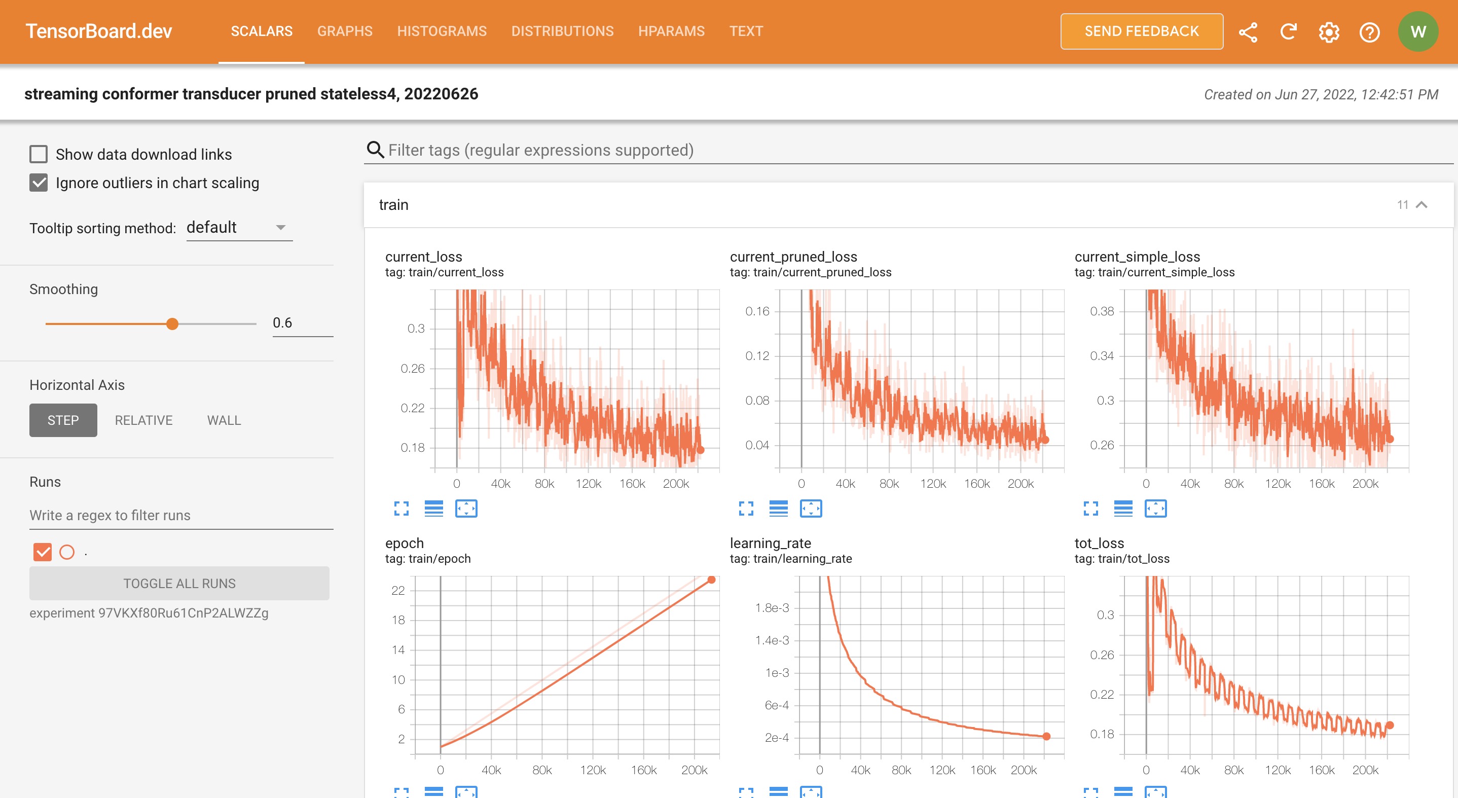
This folder contains tensorBoard logs. Training loss, validation loss, learning
rate, etc, are recorded in these logs. You can visualize them by:
$cdpruned_transducer_stateless4/exp/tensorboard
$tensorboarddevupload--logdir.--description"pruned transducer training for LibriSpeech with icefall"
It will print something like below:
TensorFlowinstallationnotfound-runningwithreducedfeatureset.Uploadstartedandwillcontinuereadinganynewdataasit's added to the logdir.Tostopuploading,pressCtrl-C.Newexperimentcreated.ViewyourTensorBoardat:https://tensorboard.dev/experiment/97VKXf80Ru61CnP2ALWZZg/[2022-11-20T15:50:50]Startedscanninglogdir.Uploading4468scalars...[2022-11-20T15:53:02]Totaluploaded:210171scalars,0tensors,0binaryobjectsListeningfornewdatainlogdir...
Note there is a URL in the above output. Click it and you will see
the following screenshot:
The decoding part uses checkpoints saved by the training part, so you have
to run the training part first.
Hint
There are two kinds of checkpoints:
(1) epoch-1.pt, epoch-2.pt, …, which are saved at the end
of each epoch. You can pass --epoch to
pruned_transducer_stateless4/decode.py to use them.
(2) checkpoints-436000.pt, epoch-438000.pt, …, which are saved
every --save-every-n batches. You can pass --iter to
pruned_transducer_stateless4/decode.py to use them.
We suggest that you try both types of checkpoints and choose the one
that produces the lowest WERs.
Tip
To decode a streaming model, you can use either simulatestreamingdecoding in decode.py or
realstreamingdecoding in streaming_decode.py, the difference between decode.py and
streaming_decode.py is that, decode.py processes the whole acoustic frames at one time with masking (i.e. same as training),
but streaming_decode.py processes the acoustic frames chunk by chunk (so it can only see limited context).
Note
simulatestreamingdecoding in decode.py and realstreamingdecoding in streaming_decode.py should
produce almost the same results given the same --decode-chunk-size and --left-context.
shows the options for decoding.
The following options are important for streaming models:
--simulate-streaming
If you want to decode a streaming model with decode.py, you MUST set
--simulate-streaming to True. simulate here means the acoustic frames
are not processed frame by frame (or chunk by chunk), instead, the whole sequence
is processed at one time with masking (the same as training).
--causal-convolution
If True, the convolution module in encoder layers will be causal convolution.
This is MUST be True when decoding with a streaming model.
--decode-chunk-size
For streaming models, we will calculate the chunk-wise attention, --decode-chunk-size
indicates the chunk length (in frames after subsampling) for chunk-wise attention.
For simulatestreamingdecoding the decode-chunk-size is used to generate
the attention mask.
--left-context
--left-context indicates how many left context frames (after subsampling) can be seen
for current chunk when calculating chunk-wise attention. Normally, left-context should equal
to decode-chunk-size*num-left-chunks, where num-left-chunks is the option used
to train this model. For simulatestreamingdecoding the left-context is used to generate
the attention mask.
The following shows two examples (for the two types of checkpoints):
shows the options for decoding.
The following options are important for streaming models:
--decode-chunk-size
For streaming models, we will calculate the chunk-wise attention, --decode-chunk-size
indicates the chunk length (in frames after subsampling) for chunk-wise attention.
For realstreamingdecoding, we will process decode-chunk-size acoustic frames at each time.
--left-context
--left-context indicates how many left context frames (after subsampling) can be seen
for current chunk when calculating chunk-wise attention. Normally, left-context should equal
to decode-chunk-size*num-left-chunks, where num-left-chunks is the option used
to train this model.
--num-decode-streams
The number of decoding streams that can be run in parallel (very similar to the bathsize).
For realstreamingdecoding, the batches will be packed dynamically, for example, if the
num-decode-streams equals to 10, then, sequence 1 to 10 will be decoded at first, after a while,
suppose sequence 1 and 2 are done, so, sequence 3 to 12 will be processed parallelly in a batch.
Note
We also try adding --right-context in the real streaming decoding, but it seems not to benefit
the performance for all the models, the reasons might be the training and decoding mismatch. You
can try decoding with --right-context to see if it helps. The default value is 0.
The following shows two examples (for the two types of checkpoints):
modified_beam_search : It implements the same algorithm as beam_search above, but it
runs in batch mode with --max-sym-per-frame=1 being hardcoded.
fast_beam_search : It implements graph composition between the output log_probs and
given FSAs. It is hard to describe the details in several lines of texts, you can read
our paper in https://arxiv.org/pdf/2211.00484.pdf or our rnnt decode code in k2. fast_beam_search can decode with FSAs on GPU efficiently.
fast_beam_search_LG : The same as fast_beam_search above, fast_beam_search uses
an trivial graph that has only one state, while fast_beam_search_LG uses an LG graph
(with N-gram LM).
fast_beam_search_nbest : It produces the decoding results as follows:
Use fast_beam_search to get a lattice
Select num_paths paths from the lattice using k2.random_paths()
Unique the selected paths
Intersect the selected paths with the lattice and compute the
shortest path from the intersection result
The path with the largest score is used as the decoding output.
fast_beam_search_nbest_LG : It implements same logic as fast_beam_search_nbest, the
only difference is that it uses fast_beam_search_LG to generate the lattice.
Note
The supporting decoding methods in streaming_decode.py might be less than that in decode.py, if needed,
you can implement them by yourself or file a issue in icefall .
Checkpoints saved by pruned_transducer_stateless4/train.py also include
optimizer.state_dict(). It is useful for resuming training. But after training,
we are interested only in model.state_dict(). You can use the following
command to extract model.state_dict().
# Assume that --epoch 25 --avg 3 produces the smallest WER# (You can get such information after running ./pruned_transducer_stateless4/decode.py)epoch=25avg=3
./pruned_transducer_stateless4/export.py\--exp-dir./pruned_transducer_stateless4/exp\--streaming-model1\--causal-convolution1\--bpe-modeldata/lang_bpe_500/bpe.model\--epoch$epoch\--avg$avg
Caution
--streaming-model and --causal-convolution require to be True to export
a streaming model.
It will generate a file ./pruned_transducer_stateless4/exp/pretrained.pt.
Hint
To use the generated pretrained.pt for pruned_transducer_stateless4/decode.py,
you can run: